Background
This article will focus on sorting algorithms including :
Table 1 : Comparison based sorting algorithm
| Algorithm | Best | Average | Worst | Space |
|---|---|---|---|---|
| Bubble | Ω ( n2 ) | Θ ( n2 ) | O ( n2 ) | O ( 1 ) |
| Selection | Ω ( n2 ) | Θ ( n2 ) | O ( n2 ) | O ( 1 ) |
| Insertion | Ω ( n ) | Θ ( n2 ) | O ( n2 ) | O ( 1 ) |
| Shellsort | Ω ( log n ) Ω ( log2 n ) | — | O ( n2 ) O ( log n ) | O ( n ) |
| Merge | Ω ( n log n ) | Θ ( n log n ) | O ( n log n ) | O ( n ) |
| Heap | Ω ( n log n ) | Θ ( n log n ) | O ( n log n ) | O ( 1 ) |
| Quicksort | Ω ( n log n ) | Θ ( n log n ) | O ( n2 ) O ( n log n ) | O ( log n ) |
Table 2 : Non-comparison based sorting algorithm
| Algorithm | Best | Average | Worst | Space |
|---|---|---|---|---|
| Count | Ω ( n + k ) | Θ ( n + k ) | O ( n + k ) | O ( n + k ) |
| Bucket | Ω ( n + k ) | Θ ( n + n2/k + k ) | O ( n2 ) | O ( n ) |
| Radix | Ω ( nk ) | Θ ( nk ) | O ( nk ) | O ( n + k ) |
Analysis of different sorting techniques
Bubble
This is the simplest sorting algorithmBubble Sort will go from one end to another performing compare & swap between the two consecutive values until all values are sorted.
Here are some of the rules used in our sorting :
- Every set of iteration will always start from one end. In our case, we will select the left or the first index to begin with.
- For vector {a, b} :
- if a ≥ b : then the index will point to the index of a
- if a < b : then they will swap and become {b, a}
PS : of course, you can always go from left to right so long you know what you are doing.
Demo
Here is a simple demo showing how Bubble Sort can sort an array [ 5, 9, 3, 1, 2, 8, 4, 7, 6 ] in ascending order.
- [ 5, 9, 3, 1, 2, 8, 4, 7, 6 ] → ( compare 5, 9 )
- [ 5, 9, 3, 1, 2, 8, 4, 7, 6 ] → ( since 5 < 9 → nothing is done )
- [ 5, 9, 3, 1, 2, 8, 4, 7, 6 ] → ( compare 9, 3 )
- [ 5, 3, 9, 1, 2, 8, 4, 7, 6 ] → ( swap 3, 9 )
- [ 5, 3, 1, 9, 2, 8, 4, 7, 6 ] → ( compare 9, 1 → swap 1, 9 )
- [ 5, 3, 1, 2, 9, 8, 4, 7, 6 ] → ( compare 9, 2 → swap 2, 9 )
- [ 5, 3, 1, 2, 8, 9, 4, 7, 6 ] → ( compare 9, 8 → swap 8, 9 )
- [ 5, 3, 1, 2, 8, 4, 7, 6, 9 ] → ( after few more compare and swap, 9 will be placed at the end )
After this, do the same thing again :
- [ 5, 3, 1, 2, 8, 4, 7, 6, 9 ]
- [ 3, 5, 1, 2, 8, 4, 7, 6, 9 ]
- [ 3, 1, 5, 2, 8, 4, 7, 6, 9 ]
- [ 3, 1, 2, 5, 8, 4, 7, 6, 9 ]
- [ 3, 1, 2, 5, 8, 4, 7, 6, 9 ]
- [ 3, 1, 2, 5, 4, 8, 7, 6, 9 ]
- [ 3, 1, 2, 5, 4, 7, 8, 6, 9 ]
- [ 3, 1, 2, 5, 4, 7, 6, 8, 9 ]
- … skip to result
By the end, we will get : [ 1, 2, 3, 4, 5, 6, 7, 8, 9 ]
PsudoCode
for i from n to 2 {
    for j from 1 to i - 1 {
        if (nums[j] > nums[j+1]) {
            int temp = nums[j + 1];
            nums[j + 1] = nums[j];
            nums[j] = temp;
        }
    }
}
What this code does is that it will perform swap whenever it finds a value at $[j]$ is greater than the next value.
We only reaches the $2^{nd}$ index on the outer loop because once values from $2..n$ are sorted, so will the $1^{st}$ one.
Time Complexity
We will calculate the time complexity using the psudocode.
| line | code | cost | # of runs |
|---|---|---|---|
| 1 | for i from n to 2 | \(c_1\) | n - 1 |
| 2 | for j from 0 to i - 1 | \(c_2\) | \(\sum_{i = 1}^{n-1}m_i\) |
| 3 | if ( nums[ j ] > nums [ j+1 ] ) | \(c_3\) | \(\sum_{i=2}^{n}(m_i -1)\) |
| 4 | swap | c_4 | \(\sum_{i=2}^{n}(m_i -1)\) |
By summing up :
\[\begin{aligned} T(n) = &c_1(n - 1) + c_2\sum_{i = 1}^{n-1}m_i + \\&c_3\sum_{i=1}^{n-1}(m_i -1) +c_4\sum_{i=1}^{n-1}(m_i -1) \end{aligned}\]Here, $c_3$ is the cost to compare and $c_4$ is the cost to swap.
Best Case
In the Best-case, all values are sorted, meaning that no swapping will be made even though both inner and outer loops will go through all values.
Here,
\[m_i = i-1 = i\]Hence :
\[\begin{aligned}\sum_{i=1}^{n-1}m_i &= \sum_{i=1}^{n-1}(i - 1) + 1 \\&= \frac{n(n-1)}{2} + 1\end{aligned}\]
NOTE : the $+1$ at the end is because the for-loop needs an extra step to exit the loop.
and
\[\begin{aligned}\sum_{i=1}^{n-1}(m_i - 1) &= \sum_{i=1}^{n-1}(i - 1) \\&= \sum_{i=1}^{n-2}i \\&= \frac{(n - 1)(n-2)}{2}\end{aligned}\]Therefore, in Best-case, we ignore $c_4$ because no swapping is performed, and we’ll get :
\[\begin{aligned} T(n) = &n^2(\frac{c_2}{2} + \frac{c_3}{2}) + \\&n(c_1 - \frac{c_2}{2} - \frac{3c_3}{2}) - \\& ( c_1 - c_2 - c_3) \end{aligned}\]As a result, in the Best-case :
- The overall complexity is $Ω(n^2/2)$
- Comparison also has the complexity of $Ω(n^2/2)$
- Swapping has a complexity of $Ω(0)$
PS : in complexity we usually don’t need to include the constants, but here we leave it be for us to compare the time complexities of comparison and swapping among the cases.
Worst Case
In the Worst-case, all values are reversed, so swapping needs to be done for $(i-1)$ times.
As you should have noticed, the only difference between Best and Worst cases is that we need to take $c_4$ into consideration.
So, the Worst-case will have the same complexity as before :
- The overall complexity is $O(n^2/2)$
- Comparison also has the complexity of $O(n^2/2)$
- Swapping also shares the same complexity of $O(n^2/2)$
Average Case
In Average Case, we expects that half of the pairs needs to be swapped.
Thus, the sums become :
\[\begin{aligned} T(n) = &c_1(n - 1) + c_2\sum_{i = 1}^{n-1}m_i + \\&c_3\sum_{i=1}^{n-1}(m_i -1) +\frac{c_4}{2}\sum_{i=1}^{n-1}(m_i -1) \end{aligned}\]which is almost the same as Worst-case :
- The overall complexity is $O(n^2/2)$
- Comparison also has the complexity of $O(n^2/2)$
- Swapping also shares the same complexity of $O(n^2/4)$
Find Big-O faster
Maybe you might be thinking, do we need to go through these tedious work just to find the complexity ?
Well, we can simplify or estimate it by multiplying the maximum times the inner and outer loops will run :
\[T(n)\approx(n - 1)(n - 2) = O(n^2)\]Space Complexity
Since Bubble Sort is arranging values inside the array, there is no extra memory being used, thus the space complexity is $O(1)$.
Optimization
For now, the best case and the worst case share the same order of complexity, but we can still optimize it.
We would hope that if the array is already sorted or if the value is already in the right place, then there’s no point of going through the inner loop more than once.
So how do we do that ? A simple flag would do.
for i from n to 2 {
    bool swapped = false;
    for j from 0 to i - 1 {
        if (nums[j] > nums[j+1]) {
            int temp = nums[j + 1];
            nums[j + 1] = nums[j];
            nums[j] = temp;
            swapped = true;
        }
    }
    if (!swapped) break;
}
With the help of swapped flag, the inner loop will break when nums[j] > nums[j+1] is always false, meaning all values are sorted already.
Now if we analysis it again :
\[\begin{aligned} T(n) = &c_1(n - 1) + c_2(n-2) \end{aligned}\]This is what we’ll get, because the inner loop will only enter $(n-2)$ times, thus resulting a complexity of $\Omega(n)$.
But this will only improve the best and the average complexity.
Epcot Center
TEST
Source Code
CPP ( Iteration )
using namespace std;
#include <vector>

// Iteration
void iteratorSort(vector<int> &nums) {
    // improved
    for (int i = nums.size() ; i > 0 ; i--) {
        bool swapped = false;
        for (int j = 0 ; j < i - 1 ; j++) {
            if (nums[j] > nums[j+1]) {
                swapped = true;
                swap(nums, j+1, j);
            }
        }
        if (!swapped) break;
    }

    static void swap(vector<int>& nums, int indexA, int indexB) {
        int a = nums[indexA];
        nums[indexA] = nums[indexB];
        nums[indexB] = a;
    }
}
CPP ( Recursive )
static void recursiveSort(vector<int> &nums, int i) {
    int t_index = nums.size() - 1;

    if (i == nums.size() - 1) return;

    bool swapped = false;

    for (int j = 0 ; j < i - 1 ; j++) {
        if (nums[j] > nums[j+1]) {
            swapped = true;
            swap(nums, j, j+1);
        }
    }

    if (!swapped) return;
    recursiveSort(nums, --i);
}
NOTE : A swap consist of 3 operations (read, write, write)
Selection
Selection Sort is quite similar to Bubble Sort, where they both has a Big-O of O( n2 ).
The main difference between the two is how many times compare and swap are performed.
In Selection Sort, instead of performing compare and swap for every value, it will do the followings:
- Find the minimum from the unsorted array
- Swap the minimum with the smallest index in the sorted array.
Simply continue performing step 1 and 2 till all values are sorted.
PS : if you are trying sort it into decending order, you can find the maximum instead.
Demo
Here is a simple demo showing how Selection Sort can sort an array [ 5, 9, 3, 1, 2, 8, 4, 7, 6 ] in ascending order.
- [ 5, 9, 3, 1, 2, 8, 4, 7, 6 ] → (scan for min)
- [ 1, 9, 3, 5, 2, 8, 4, 7, 6 ] → (swap with index 0)
- [ 1, 9, 3, 5, 2, 8, 4, 7, 6 ] → (scan for min)
- [ 1, 2, 3, 5, 9, 8, 4, 7, 6 ] → (swap with index 1)
- … skip to result
By the end, we will get : [ 1, 2, 3, 4, 5, 6, 7, 8, 9 ]
PsudoCode
for i in 1 to n - 1 {
    int target = i;
    for j in i + 1 to n {
        if (nums[target] > nums[j]) {
            target = j;
        }
    }
    // swap
    int temp = nums[i];
    nums[i] = nums[target];
    nums[target] = temp;
}
Time Complexity
Again, with similar process as before, we will get the followings :
\[\begin{aligned} T(n) = &c_1(n - 1) + c_2(n-2) + c_3\sum_{i = 2}^{n}m_i + \\&c_4\sum_{i = 2}^{n}(m_i - 1) + c_5\sum_{i = 2}^{n}(m_i - 1) + \\\\&(c_6 + c_7 + c_8)(n - 2) \end{aligned}\]By examining the formula, we can see that in both best and worst cases have an order magnitude of 2 or $\Omega(n^2)$ and $O(n^2)$ respectively.
This is also the case for both comparison and swap.
Space Complexity
Again, there is no extra memory used for this sorting, except for the local variables, so it also has a complexity of $O(1)$.
Optimization
Just like Bubble Sort, we might want the loops to end early. So how can we do it ?
for i in 1 to n - 1 {
    int target = i;
    for j in i + 1 to n {
        if (nums[target] > nums[j]) {
            target = j;
        }
    }
    // swap only if needed
    if (target != i) {
        int temp = nums[i];
        nums[i] = nums[target];
        nums[target] = temp;
    }
}
Unlike Bubble Sort that only needs to go through the inner loop $n - 1$ times to tell if the array is already sorted, Selection Sort cannot do so.
This is because Selection Sort only check if there are values smaller than the target index, meaning that you have to go through the whole array just to be sure that the array is not sorted.
Take [ 1, 2, 3, 4, 6, 5 ] for example, we will only know that 6 and 5 are reversed when the $5^{th}$ index becomes our target of interest.
As a result, after optimization, the order of magnitude of the complexity has not changed, but the complexity for comparison and swap have.
Before optimization, in the best-case, swapping has a complexity of $\Omega(n^2)$. But now, in the best-case, its complexity becomes $\Omega(0)$.
Source Code
C++
void sort(vector<int> &nums, bool iteration) {
    for(int i = 0 ; i < nums.size() - 1 ; i++) {

        int min_index = i;

        for (int j = i + 1 ; j < nums.size() ; j++) {
            if (nums[j] < nums[min_index]) {
                min_index = j;
            }
        }

        if (min_index != i) {
            int min = nums[min_index];
            nums[min_index] = nums[i];
            nums[i] = min;
        }
    }
}
What has improved ?
Compared to Bubble Sort, Selection Sort has the following advantage :
- Less computation Instead of performing compare and swap for every values, Selection Sort also compare every values, but only perform n times of swap in total.
Insertion
Insertion Sort also has a time complexity of O ( n2 ), but instead of using comparison and swapping, like Bubble Sort, it uses comparison and moving instead.Since swapping requires 3 operations while moving only takes 1 operation, Insertion Sort is expected to be faster than Bubble and Selection Sort.
Here is how Insertion Sort is done :
- Select the value at index 0 as the sorted ( left ) array initial value.
- Select the next value on the right and insert into the left array through shift and insert.
The rest of the process will simply repeat step 2 until the right array is empty.
Also, what Insertion Sort is doing here is called divide and conquer, though we only divided the array into 2 pieces.
Just to help you understand the operation of Insertion Sort, just think of how do you sort your cards while playing poker.
Demo
Here is a simple demo showing how Insertion Sort can sort an array [ 5, 9, 3, 1, 2, 8, 4, 7, 6 ] in ascending order.
- [ 5, 9, 3, 1, 2, 8, 4, 7, 6 ] → ( pick 5 as the inital value )
- [ 5, 9, 3, 1, 2, 8, 4, 7, 6 ] , [9] → ( holds 9 ; compare 9 and 5 )
- [ 5, 9, 3, 1, 2, 8, 4, 7, 6 ] , [3] → (holds 3 ; compare 3 with 9)
- [ 5, 9, 9, 1, 2, 8, 4, 7, 6 ] , [3] → (since 9 > 3, shift 9 to the right )
- [ 5, 5, 9, 1, 2, 8, 4, 7, 6 ] , [3] → ( since 5 > 3 , shift 5 to the right )
- [ 3, 5, 9, 1, 2, 8, 4, 7, 6 ] → ( place 3 back to array )
- [ 3, 5, 9, 1, 2, 8, 4, 7, 6 ] , [1] → (holds 1 ; compare 1 and 9)
- … skip to result
Now you should be able to understand how Insertion Sort is done, the final result should be [ 1, 2, 3, 4, 5, 6, 7, 8, 9 ]
PsudoCode
Here are something to keep in mind :
- The inital value of the sorted array is always index 0, hence we can skip this index when defining the sub-array.
- The outer loop should end when all values have been looped.
- The inner loop should end when value has inserted at the right location.
for i in 2 to n {
  int target = nums[i];
  int j = i - 1;
  while (j > 0 && nums[j] > t) {
    nums[j + 1] = nums[j];
    j--;
  }

  nums[j + 1] = target;
}
Time Complexity
By examining the psudocode, we can come up with a fomula :
\[\begin{aligned} T(n) = &c_1(n - 1) + (c_2 + c_3)(n-2) +\\ &c_4\sum_{i = 2}^{n}m_i + (c_5 + c_6)\sum_{i = 2}^{n}(m_i-1) +\\&c_7(n - 2) \end{aligned}\]Best Case
In the Best-case, the array should be sorted already, ie [ 1, 2, 3, 4, 5, 6 ].
Next, we need to find out what is the value of $m_i$. To do so, we need to answer this question :
If we feed this array into the function, how many time will the while-loop runs ?
Obviously, it will try to enter the loop once, because it will be stopped when comparing nums [ j ] with t.
Resulting :
\[m_i = 1\]And since it won’t run the content of the while loop, $T(n)$ becomes :
\[\begin{aligned} T(n) = &c_1(n - 1) + (c_2 + c_3)(n-2) +\\ &c_4\sum_{i = 2}^{n}1 +c_7(n - 2) \\\\= &c_1(n - 1) + (c_2 + c_3)(n-2) +\\ &c_4(n-2) +c_7(n - 2) \\\\=&n(c_1 + c_2 + c_3 + c_4 + c_7) - \\&(c_1 +2c_2 + 2c_3 + 2c_4 + 2c_7) \end{aligned}\]As a result, we can say that :
- In best-case, the time complexity is $\Omega(n)$
- The time complexity of comparison is $\Omega(n)$
- The time complexity of moving is $\Omega(n)$
And to be more specific, because there are only 2 moving and comparison operations in best-case, so we can also say that :
- The time complexity of moving and comparison are $\Omega(2(n-1)) = \Omega(2n-2)$
Worst Case
In the worst-case, the array is reversed to begin with.
In this case, the while loop will run $(i-1)$ times, thus :
\[\begin{aligned} \sum_{i=2}^{n}m_i &= \sum_{i=2}^{n}(i-1) + 1 \\&= \sum_{i=2}^{n}i \\&= \sum_{i=1}^{n}i - 1 \\&= \frac{(n+1)(n)}{2} - 1 \\&= \frac{n^2 + n - 2}{2} \\&= \frac{(n-1)(n+2)}{2} \end{aligned}\] \[\begin{aligned} \sum_{i=2}^{n}(m_i - 1) &= \sum_{i=2}^{n}(i-2) \\&= \sum_{i=1}^{n-2}i \\&= \frac{(n-1)(n-2)}{2} \end{aligned}\]As a result, $T(n)$ becomes :
\[\begin{aligned} T(n) = &c_1(n - 1) + (c_2 + c_3)(n-2) +\\ &c_4\frac{(n - 1)(n + 2)}{2} + \\&(c_5 + c_6)\frac{(n-1)(n-2)}{2} +\\&c_7(n - 2) \\\\=&\frac{n^2}{2}(c_4 + c_5 + c_6) + \\&n(c_1 + c_2 + c_3 + \frac{c_4}{2} - \frac{3c_5}{2} - \frac{3c_6}{2} + c_7) - \\&(c_1 + 2c_2 + 2c_3 - c_5 - c_6 + 2c_7) \end{aligned}\]Therfore, the time complexities for worst case are :
- Total time complexity is $O(n^2/2)$
Comparison time complexity is
\[O(\frac{(n-1)(n+2)}{2}) \approx O(\frac{n^2}{2})\]Moving time complexity is
\[\begin{aligned} &O(2(n-1) + \frac{(n)(n-1)}{2}) \\=&O(\frac{n^2 - n + 4n - 4}{2}) \\=&O(\frac{n^2+ 3n - 4}{2}) \\\approx &O(\frac{n^2}{2}) \end{aligned}\]
Space Complexity
Same as before, since no extra memory is used, the space complexity is $O(1)$.
Optimization
How can we optimize this algorithm ?
Actually, there is nothing that you can do to optimize this algorithm anymore.
Source Code
C++ ( Iteration )
static void iterationSortWithWhile(vector<int>& nums) {
    for (int i = 1 ; i < nums.size() ; i++) {
      int t = nums[i];
      int j = i - 1;

      while (j > 0 && nums[j] > t) {
        nums[j + 1] = nums[j];
        j--;
      }

      nums[j + 1] = t;
    }
}

// you can also use for-loop instead :
static void iterationSort(vector<int>& nums) {
    for (int i = 1 ; i < nums.size() ; i++) {
        int t = nums[i];
        for (int j = i ; j > 0 ; j--) {
            if (nums[j - 1] > t) {
                nums[j] = nums[j - 1];
            } else {
                nums[j] = t;
                break;
            }

            if (j - 1 == 0) {
                nums[j - 1] = t;
                break;
            }
        }
    }
}
C++ ( Recursive )
// Recursive can take care the first for-loop
static void recursiveSort(vector<int>& nums, int i = 1) {
    if (i == nums.size()) return;
    int t = nums[i];
    int j = i;

    while (j != 0) {
        if (nums[j - 1] > t) {
            nums[j] = nums[j - 1];
            j--;
        } else {
            break;
        }
    }

    nums[j] = t;

    recursiveSort(nums, i+1);
}
What has improved ?
Comparing to Bubble and Selection, instead of using swap, which takes 3 operations (read, write, write), Insertion Sort uses shift, which only needs to perform a single write operation.
Thus, Insertion is more efficient than the previous two.
However, to make Insertion Sort more efficient, we can look into Shellsort, which is an optimized version of Insertion Sort.
Shell Sort
Shellsort is quite an interesting sorting algorithm. It is an unstable and in-place comparison sort that is a generalized version of Insertion Sort.
As we recall from Insertion Sort, whenever we find a value that is smaller than the sorted subarray, we need to shift the sorted values one step at a time. Thus, in the worst case, we will get $O(n^2)$ complexity.
However, what if we can shift more steps at a time ? That should help us reduce some computational time, especially for extremity values.
In order to do so, Shellsort uses gaps ( h ) to pair up values to perform comparison.
[ 5, 9, 3, 1, 2, 8, 4, 7, 6 ] h = 4
  5 --------- 2               5 > 2 ... swap
     9 --------- 8            9 > 8 ... swap
        3 --------- 4         3 < 4 ... x
           1 --------- 7      1 < 7 ... x
                          6
// result
[ 2, 8, 3, 1, 5, 9, 4, 7, 6 ]
Now that the array is sorted with gap of 4, we say that the resulting array is 4-sorted. And in general, we call these array h-sorted.
After the array become h-sorted, we need to decrease h by half and sort it again, until h becomes 1, which will become a Insertion Sort or Bubble Sort.
So the steps involved are :
- pick a h value as the initial gap
- make array h-sorted
- divide h by half and repeat step 1.
Demo
Let’s keep sorting [ 5, 9, 3, 1, 2, 8, 4, 7, 6 ] with Shellsort.
- select $h = 9 / 2 \approx{4}$
[ 5, 9, 3, 1, 2, 8, 4, 7, 6 ] h = 4 5 --------- 2 --------- 6 do insertion sort 9 --------- 8 9 > 8 ... swap 3 --------- 4 3 < 4 ... x 1 --------- 7 1 < 7 ... x // after sorting [ 2, _, _, _, 5, _, _, _, 6 ] [ _, 8, _, _, _, 9, _, _, _ ] [ _, _, 3, _, _, _, 4, _, _ ] [ _, _, _, 1, _, _, _, 7, _ ] // result [ 2, 8, 3, 1, 5, 9, 4, 7, 6 ] - set $h = 4 / 2 = 2$
[ 2, 8, 3, 1, 5, 9, 4, 7, 6 ] h = 2 2 --- 3 --- 5 --- 4 --- 6 do insertion sort 8 --- 1 --- 9 --- 7 do insertion sort // after sorting [ 2, _, 3, _, 4, _, 5, _, 6 ] [ _, 1, _, 7, _, 8, _, 9, _ ] // result [ 2, 1, 3, 7, 4, 8, 5, 9, 6 ] - set $h = 1$, meaning we will perform insertion sort on the whole array
 [ 2, 1, 3, 7, 4, 8, 5, 9, 6 ] h = 1

 // result
 [ 1, 2, 3, 4, 5, 6, 7, 8, 9 ]
PsudoCode
void sort(int arr[]) {
    int n = sizeof(arr)/sizeof(arr[0]);
    int gap = n / 2;

    while(gap >= 1) {
        int groups = n / gap;
        for i from 0 to groups {
            insertSort(arr, i, gap);
        }
    }
}

void insertSort(int arr[], int start, int gap) {
    int n = sizeof(arr)/sizeof(arr[0]);
    for (int i = start + gap; i < n; i += gap) {
        int currentValue = arr[i];
        int currentIndex = i;

        for (int j = i - gap; j >= start; j -= gap) {
            if (arr[j] > currentValue) {
                arr[currentIndex] = arr[j];
                currentIndex = j;
            }
        }

        if (currentIndex != i) {
            arr[currentIndex] = currentValue;
        }
    }
}
Time Complexity
From Insertion Sort, we know that the worst time complexity is $O(n^2)$, which is also the worst time complexity of Shellsort.
However, in the best case, when the initial array is already sorted, the time complexity is $O(nlog(n))$.
This is because even though all values are sorted, we still need to go through the gap sequence :
\[n/2 , n/2^2 , ... , 1\]Since it will take $log(n)$ steps to reach 1 :
\[\begin{aligned} &\frac{n}{2} + \frac{n}{2^2} + ... + \frac{n}{2^{log(n)}} \\\\= &\frac{n}{2} + \frac{n}{2^2} + ... + 1 \\\\= &\sum_{i = 1}^{log(n)} \frac{n}{2^i} \\\\= &nlog(n) \text{ ... (Harmonic Series)} \end{aligned}\]Space Complexity
Since this is a in-place sorting algorithm, just like Insertion Sort, its space complexity is $O(1)$.
Other Gap sequences
The gap sequence that is used to demostrate Shellsort is proposed by Donald Shell in 1959 with a sequence of :
\[(\frac{n}{2}, \frac{n}{4}, \frac{n}{8} ..., 1)\]But, that’s not the only gap sequence that had been proposed and it is definely not the best gap sequence there is.
Here a list of gap sequences that has been proposed over the years.
Perhaps we could have more discussion on this topic in the future.
Source Code
C++ Iterative
void iterativeSort(vector<int>& nums) {
    int n = nums.size();
    int gap = n / 2;

    while(gap >= 1) {
        int groups = n / gap;

        for (int i = 0; i <= groups; i ++ ){
            iterativeInsertSort(nums, i, gap);
        }

        gap = gap / 2;
    }
}

void iterativeInsertSort(vector<int>& nums, int start, int gap) {
    int n = nums.size();

    for (int i = start + gap; i < n; i += gap) {
        int currentValue = nums[i];
        int currentIndex = i;

        for (int j = i - gap; j >= start; j -= gap) {
            if (nums[j] > currentValue) {
                nums[currentIndex] = nums[j];
                currentIndex = j;
            }
        }

        if (currentIndex != i) {
            nums[currentIndex] = currentValue;
        }

    }
}
What has improved ?
By separating the input into subarrays, Shellsort has improved the time complexity in best case from $O(n)$ to $O(log(n))$.
Even though under Shell’s gap sequence, the worst case time complexity is still $O(n^2)$, but it can be improved by choosing other gap sequences.
Resources
- wiki
- YT : Sorts 5 Shell Sort
- Shell Sort Algorithm: Everything You Need to Know
- stackoverflow: Time Complexity
Merge Sort
In the algorithms we’ve seen so far ( Bubble, Selection and Insertion Sort ) , they are mainly suitable for small data set. As the size of the data grows, their efficiency ($O(n^2)$) will raise exponentially.
So is there anything we can do to increase the efficiency in sorting a large data set ?
Perhaps if we can chops the data into smaller pieces and sort them before merging them together ?
This is exactly what Merge Sort does.
Merge Sort uses divide and conquer to divide large data set into smaller chuncks. After sorting these chuncks they will be merged into a larger sorted chuncks.Through these processes, the whole data will become sorted at the end through merging, hence the name Merge Sort.
Here is how Merge Sort is done :
- divide the array into n number of arrays with 1 item per array.
- merge 2 adjacent arrays together by picking out the smaller value and insert it into a new array, until all items are inserted into the array.
By continuing step 2, the array will be sorted at the end.
Demo
Here we’ll use Merge Sort to sort the following array :
[ 5, 9, 3, 1, 2, 8, 4, 7, 6 ]
- divide the array till all array contains only 1 item
- [ 5, 9, 3, 1, 2, 8, 4, 7, 6 ]
- [ 5, 9, 3, 1, 2 ] [ 8, 4, 7, 6 ]
- [ 5, 9, 3 ] [ 1, 2 ] [ 8, 4 ] [ 7, 6 ]
- [ 5, 9 ] [ 3 ] [ 1 ] [ 2 ] [ 8 ] [ 4 ] [ 7 ] [ 6 ]
- [ 5 ] [ 9 ] [ 3 ] [ 1 ] [ 2 ] [ 8 ] [ 4 ] [ 7 ] [ 6 ]
- start marging each array with its adjacent array
- [ 5 ] [ 9 ] [ 3 ] [ 1 ] [ 2 ] [ 8 ] [ 4 ] [ 7 ] [ 6 ]
- [ 5, 9 ] [ *1, *3 ] [ 2, 8 ] [ 4, 7 ] [ 6 ]
- [ 1, 3, 5, 9 ] [ 2, 4, 7, 8 ] [ 6 ]
- [ 1, 2, 3, 4, 5, 7, 8, 9 ] [ 6 ]
- [ 1, 2, 3, 4, 5, 6, 7, 8, 9 ]
The whole process looks like this :
                    { 5, 9, 3, 1, 2, 8, 4, 7, 6 }
                    ┌-------------┴--------------┐

            { 5, 9, 3, 1, 2 }              { 8, 4, 7, 6 }
            ┌-------┴-------┐              ┌------┴------┐

       { 5, 9, 3 }       { 1, 2 }      { 8, 4 }       { 7, 6 }
      ┌-----┴-----┐      ┌--┴--┐       ┌--┴--┐        ┌--┴--┐

  { 5, 9 }      { 3 }  { 1 } { 2 }   { 8 } { 4 }    { 7 } { 6 }
  ┌--┴--┐         |      |     |       |     |        |     |

{ 5 } { 9 }     { 3 }  { 1 } { 2 }   { 8 } { 4 }    { 7 } { 6 }

  └--┬--┘         └--┬--┘      └---┬---┘     └---┬---┘      |
  { 5, 9 }       { 1, 3 }      { 2, 8 }       { 4, 7 }    { 6 }

     └------┬-------┘              └------┬------┘          |
      { 1, 3, 5, 9 }                { 2, 4, 7, 8 }        { 6 }

            └---------------┬--------------┘                |
                { 1, 2, 3, 4, 5, 7, 8, 9 }                { 6 }

                             └----------------┬-------------┘
                                { 1, 2, 3, ,4 ,5, 6, 7, 8, 9 }
Understanding the Process
Before we start writing our psudocode, let’s take a moment to try to understand what had happened during Merge Sort. This will give us a cleaner picture when we are solving this problem.
Dividing
In this process, the initial array will be divided into smaller chuncks. This process will continue until all chuncks contains only single item.
Since in this process the n sized array will be divided by half in every step, and if it takes x steps to complete, we can say that :
\[\begin{aligned}&\frac{n}{2^x} = 1 \\&n = 2^x \\&x = log_2{(n)} \end{aligned}\]Meaning that it will take $log{(n)}$ steps to chops the array into unit sized chuncks.
So how do we approach this ?
Here is my approach : Knowing that by the end of the division, all items will be contained in their own individual array, we can simply use a for-loop and loop through the array with a certain step size.
This way, we can skip the division steps and go directly to the merging part.
[ 5 ], [ 9 ], [ 3 ], [ 1 ], [ 2 ], [ 8 ], [ 4 ], [ 7 ], [ 6 ]

for i in 0 to n with step_size = 2
    if (i + 1 < n) {
        merge(arr, i, i + 1)
    }

[ 5, 9 ], [ 1, 3 ], [ 2, 8 ], [ 4, 7 ], [ 6 ]

for i in 0 to n with step_size = 4
    if (i + 2 < n) {
        merge(arr, i, i + 2)
    }

[ 1, 3, 5, 9 ], [ 2, 4, 7, 8 ], [ 6 ]

for i in 0 to n with step_size = 8
    if (i + 4 < n) {
        merge(arr, i, i + 4)
    }

[ 1, 2, 3, 4, 5, 7, 8, 9 ], [ 6 ]

merge(arr, 0, n - 1)

[ 1, 2, 3, 4, 5, 6, 7, 8, 9 ]
If we combine them, we’ll get something like this :
void mergeSort(int array[]) {
    int step = 2;
    int n = array.size();

    // 1. keep merging until step size > size of array
    while(n > step) {
        for i from 0 to n with increment of `step`  {
            // 2.define subarrays range
            int start = i;
            int end = i + step - 1;
            int mid = (end - start) / 2 + start;

            // 3. if end is out of range, simply move it back to the proper location
            if (end > n - 1) {
                end = n - 1;
            }

            // 4.merge subarrays with index range :
            // [i ... mid] [mid+1 .... i + step - 1]
            merge(array, start, mid, end);
        }
        // 5.starts next round of merging, the size should increament by double
        step *= 2;
    }

    // 6. do one last merge for the last two subarrays
    //    go back to the previous step to find the
    //    start index of the remainding subarray.
    step /= 2;
    if (step < n) {
        /* merge(array, 0, step - 1, n - 1); */
        // use `step` instead of `step - 1` because
        // items before `step` has already been sorted in the loop.
        merge(array, 0, step, n - 1);
    }
}
From the code, we can see that all we are doing is repeatedly calling merge(array, start, mid, end); with different start indexes from both subarray.
NOTE : We need to pass start, mid and end intomergebecause subarrays might not have the same sizes. And merging them require us to know the range of subarrays.
Therefore, we can turn the code into recursive Implementation. Also, we can replace mid with :
\[\begin{aligned} mid &= (end - start) / 2 + start \\&= (start + end) / 2 \end{aligned}\]void mergeSort(int array[], int start, int end ) {
if (start >= end) return;
int mid = (end - start) / 2 + start;
// left child
mergeSort(array, start, mid);
// right child
mergeSort(array, mid+1, end);
merge(array, start, mid, end);
}
The main differences between the two implementations are :
the number of steps to chop up the array.
Iteration assumes the array is divided into unit sized array at the beginning.
 { 5, 9 }       { 1, 3 }      { 2, 8 }       { 4, 7 }    { 6 }

    └------┬-------┘              └------┬------┘          |
     { 1, 3, 5, 9 }                { 2, 4, 7, 8 }        { 6 }

           └---------------┬--------------┘                |
               { 1, 2, 3, 4, 5, 7, 8, 9 }                { 6 }

                            └----------------┬-------------┘
                                   { 1, 2, 3, ,4 ,5, 6, 7, 8, 9 }
Whereas Recursion need to chop up the array first before performing merging.
The way the array is being divided Iteration divides subarrays from left to right. Whereas Recursion divides subarrays from center and only merge the subarrays that are in the same group.
                     { 5, 9, 3, 1, 2, 8, 4, 7, 6 }
                     ┌-------------┴--------------┐

             { 5, 9, 3, 1, 2 }              { 8, 4, 7, 6 }
             ┌-------┴-------┐              ┌------┴------┐

        { 5, 9, 3 }       { 1, 2 }      { 8, 4 }       { 7, 6 }
       ┌-----┴-----┐      ┌--┴--┐       ┌--┴--┐        ┌--┴--┐

   { 5, 9 }      { 3 }  { 1 } { 2 }   { 8 } { 4 }    { 7 } { 6 }
   ┌--┴--┐         |      |     |       |     |        |     |

 { 5 } { 9 }     { 3 }  { 1 } { 2 }   { 8 } { 4 }    { 7 } { 6 }

   └--┬--┘         |     └---┬---┘     └---┬---┘       └--┬--┘
   { 5, 9 }      { 3 }   { 1, 2 }       { 4, 8 }       { 6, 7 }

      └------┬-----┘         |        └----------┬---------┘
        { 3, 5, 9 }      { 1, 2 }         { 4, 6, 7, 8 }

             └-------┬------┘                    |
             { 1, 2, 3, 5, 9 }             { 4, 6, 7, 8 }

                     └-------------┬-------------┘
                     { 1, 2, 3, ,4 ,5, 6, 7, 8, 9 }
Merging
Now that we’ve done dealing with Dividing, we need to merge them into one.
In order to create a merged array, we need to create a new array that can hold all values :
void merge(int array[], int start, int end) {
    int mid = (end - start) / 2;
    int result[end - start + 1];
}
Then, we will compare the two sorted subarrays as follows :
left = [5, 9] , right = [1, 3] , result[4]

// compare left[0] and right[0]
5 > 1

// place 1 into result
left = [5, 9] , right = [1, 3] , result[4] = [1]

// compare left[0] and right[1]
5 > 3

// place 3 into result
left = [5, 9] , right = [1, 3] , result[4] = [1, 3]

// now that right is all inserted into the result, we just insert left into result
left = [5, 9] , right = [1, 3] , result[4] = [1, 3, 5, 9]
From above, we can tell that we need to keep track of the current indexes to be compared, thus :
void merge(int array[], int start, int mid, int end) {
    int currentIndex = 0;
    int size = end - start + 1;
    int result[size];

    int i = start;
    int j = mid + 1;

    // while both subarray has not been completely inserted into the new array
    while(i <= mid && j <= end) {
        // insert the smaller value into the new array
        // then increment the index for the corresponding subarray.
        if (array[i] < array[j]) {
            result[currentIndex] = array[i];
            i++;
        } else {
          result[currentIndex] = array[j];
          j++;
        }

        currentIndex ++;
    }

    // in case one of the subarray is done reading
    // simply put all the value from the unfinished array into result array.
    if (i <= mid) {
        for (int k = i; k <= mid; k++) {
            result[currInd] = nums[k];
            currInd++;
        }
    } else if (j <= end) {
        for (int k = j; k <= end; k++) {
            result[currInd] = nums[k];
            currInd++;
        }
    }


    // write back to original array
    for (int k = 0; k < size; k++) {
        array[k + start] = result[k];
    }
}
PsudoCode
Here we will look at the approaches to this algorithm using iteration and recursion.
From the previous section, we have already come up with a complete solution for Merge Sorting. In this section we will see a clearer picture of what those codes does.
iteration
void mergeSort(int array[]) {
  int step;
  int n = array.size();

  for (step = 2 ; step <= n ; step*=2) {
      for (int i = 0; i < n ; i += step)  {
          int start = i;
          // here we can simply use min function
          int end = min(start + step - 1, n - 1);
          int mid = min(start + step/2 - 1, n - 1);

          merge(array, start, mid, end);
      }
  }

  step /= 2;
  if (step < n) {
      merge(array, 0, step, n - 1);
  }
}
Recursion
void sortRecursively(vector<int>& nums, int start, int end) {
    if (start >= end) return;

    int mid = (end - start) / 2 + start;

    // left child
    sortRecursively(nums, start, mid);
    // right child
    sortRecursively(nums, mid+1, end);

    merge(nums, start, mid, end);
}
Merge
void merge(vector<int>& nums, int start, int mid, int end) {
    int currInd = 0;
    int size = end - start + 1;
    int result[size];
    int i = start, j = mid + 1;

    while(i <= mid && j <= end) {
        if (nums[i] < nums[j]) {
            result[currInd] = nums[i];
            i++;
        } else {
            result[currInd] = nums[j];
            j++;
        }

        currInd++;
    }

    while(i <= mid) {
        result[currInd] = nums[i];
        currInd++;
        i++;
    }

    while (j <= end) {
        result[currInd] = nums[j];
        currInd++;
        j++;
    }

    // rewrite nums values
    for k from 0 to size {
        nums[k + start] = result[k];
    }
}
Time Complexity
In order to examine time complexity of Merge Sort, we need to look at both Division and Merge separately.
Division From the code, we know that it takes 2 loops to achieve division.
The outer loop will run x times till step is greater than n. Since x is increased by multiplying by 2, so we can write :
The inner loop on the other hand will run according to the step size.
\[\begin{aligned} \text{inner loop runs} &= \sum_{i = 1}^{log_2(n)}\frac{n}{2^i} \end{aligned}\]Every time the loop runs, merge will be run once.
The process for merge is quite simple. It simply loop through all the values and performs read and write on all values. Since the number of values that will be merged is exactly the step size, we can write :
But , thus we combine the inner loop runs and merging cost to be :
\[\begin{aligned} \text{merging cost for certain step} &= \sum_{i = 1}^{log_2(n)}\frac{n}{2^i} \times 2^i \\&= n\sum_{i = 1}^{log_2(n)} 1 \\&= n\times log_2(n) \end{aligned}\]As a result, we can say that the time complexity of Merge Sort in iteration is $O(nlog(n))$.
Recursive In Recursive form, we can also get the same result. However, it is derived using different method.
Let’s take a look at the code :
void sortRecursively(vector<int>& nums, int start, int end) {
    if (start >= end) return;
    int mid = (end - start) / 2 + start;

    sortRecursively(nums, start, mid);
    sortRecursively(nums, mid+1, end);
    merge(nums, start, mid, end);
}
We can see that the code is simply calling sortRecursively repeatedly with half of the array size and merge the array with a full size of the array.
Therefore, by assuming the time it takes to run sortRecursively is $T(n)$, and the total cost to merge is $c$, we can write :
Also, when the size of the array is less than 2, it will simply return, so we can add this condition to the formula above to :
\[T(n) = \begin{cases} c_1, &\text{if n = 1} \\2T(\frac{n}{2}) + c_2n, &\text{if n > 1} \end{cases}\]where both $c_1$ and $c_2$ are assumed to be positive.
If we expand the formula :
\[\begin{aligned} T(n) &= 2T(\frac{n}{2}) + c_2n \\&= 4T(\frac{n}{4}) + 2c_2n \\&= 8T(\frac{n}{8}) + 3c_2n \\&= 2^3T(\frac{n}{8}) + 3c_2n \\& = ... \\& \text{until } 2^{log_2{n}} \\&= nT(1) + c_2nlog_2{(n)} \end{aligned}\]We can see that the time complexity is $O(nlog_2{(n)})$.
Space Complexity
The main part that uses space is whenmergeis being performed.
If we look at the merge, we can see that it simply uses an array that has the same size as the subarray. Thus :
Source Code
C++ Iteration
static void sortIterativelyCorrectly(vector<int>& nums) {

    int step = 2;
    int n = nums.size();

    if (n < 2) return;

    while(n > step) {
        for (int i = 0; i < n; i += step) {

            int start = i;
            int end = i + step - 1;
            int mid = (end - start) / 2 + start;

            if (end > n - 1) break;

            merge(nums, start, mid, end);
        }

        step *= 2;
    }

    step /= 2;

    if (step < n) {
        merge(nums, 0, step - 1, n - 1);
    }

}
C++ Recursion
static void sortRecursively(vector<int>& nums, int start, int end) {
    if (start >= end) return;

    int mid = (end - start) / 2 + start;

    // left child
    sortRecursively(nums, start, mid);
    // right child
    sortRecursively(nums, mid+1, end);

    merge(nums, start, mid, end);
}
C++ Merge
static void merge(vector<int>& nums, int start, int mid, int end) {
    int currInd = 0;
    int size = end - start + 1;
    int result[size];
    int i = start, j = mid + 1;

    while(i <= mid && j <= end) {
        if (nums[i] < nums[j]) {
            result[currInd] = nums[i];
            i++;
        } else {
            result[currInd] = nums[j];
            j++;
        }

        currInd++;
    }

    while (i <= mid) {
        result[currInd] = nums[i];
        currInd++;
        i++;
    }
    while (j <= end) {
        result[currInd] = nums[j];
        currInd++;
        j++;
    }

    for (int k = 0; k < size; k++) {
        nums[k + start] = result[k];
    }
}
What has improved ?
Obviously, through divide and conquer, Merge Sort shows a much better performance than all the algorithms we’ve seen so far.
The main improvement that is made is that Merge Sort will divide arrays into pieces, making them a smaller problem to solve. Also, though merging is a bit like Selection Sort, but since we are merging two sorted arrays, the problem becomes simpler and can be solved with higher efficiency.
Now you might be wondering what are the advantages of implementing Recursion over Iteration implementations.
Since Iterative Merge Sort skips the division parts, it is slightly faster than Recursive Merge Sort.
However, Recursive is much easier to implement.
Resources
Heap Sort
Another algorithm that is very similar to Merge Sort is Heap Sort.
Heap Sort also uses divide and conquer to sort the array. However, instead of dividing the input array into subarrays, it uses heap (a data structure) to sort the array.
What’s a Heap ?
A Heap is a special Tree-based data structure in which the tree is a complete binary tree. – geeksforgeeksA complete binary tree is a special type of binary tree where all the levels of the tree are filled completely except the lowest level nodes which are filled from as left as possible. – geeksforgeeks
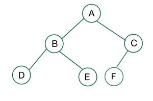
Complete Binary Tree
Heap Structure
If we look at the heap below, all nodes are labeled with the index of the array, as well as the level of the nodes.
         0----------------- Level 0
    ┌----┴----┐
    1         2 ----------- Level 1
  ┌-┴-┐     ┌-┴-┐
  3   4     5   6 --------- Level 2
┌-┴-┐
7     --------------------- Level 3
Let’s try to figure out the relationships among parent and children nodes.
| height | index(es) | # of nodes |
|---|---|---|
| 0 | 0 | $2^0$ |
| 1 | 1, 2 | $2^1$ |
| 2 | 3, 4, 5, 6 | $2^2$ |
| 3 | 7, 8, 9, 10, 11, 12, 13, 14 | $2^3$ |
By examining the table above, we can see that the relationships among node, parent and children indexes are related as follows :
| index | left index | right index | parent index |
|---|---|---|---|
| n | 2n + 1 | 2n + 2 | \(\frac{n - 1}{2}\) |
We use $n - 1$ to find the parent index because we can always round down to get the correct parent index.
Here are some tests to prove it right :
| n | left node | right node | parent |
|---|---|---|---|
| 0 | 2 x 0 + 1 = 1 | 2 x 0 + 2 = 2 | x |
| 1 | 2 x 1 + 1 = 3 | 2 x 1 + 2 = 4 | \(\frac{0}{2} = 0\) |
| 2 | 5 | 6 | \(\frac{1}{2}\approx 0\) |
| 3 | 7 | 8 | \(\frac{3 - 1}{2} = 1\) |
| 4 | 9 | 10 | \(\frac{3}{2}\approx 1\) |
| 6 | 13 | 14 | \(\frac{5}{2}\approx 2\) |
As you can see, we can now find the node’s parent and children through any given index.
Also, you might have noticed the nodes of the parents go consecutively from $0, 1, 2, … \frac{n-1}{2}$.
Other than these, there is still a lot of things that we can talk about tree and heap, but that will have to wait.
For now, you just need to know this :
- To create a tree using an array, we simply follow the array and fill the tree from top to down then from left to right [ A , B, C, D, E, F ] will give you a tree from above.
- It must follow one of the heap properties, we choose to fulfill max heap property, meaning :
- root is the largest among all nodes ie A >= all nodes
- any parent is greater than children ie B >= D or E
Next, we should see how to fulfill max heap property through a process called Heapify or Heapification.
Heapification
Let’s take [ 5, 9, 3, 1, 2, 8, 7, 6 ] as an example.
To create a tree from the array, we simply fill the tree up following the index of the array :
         5                            0 index
    ┌----┴----┐                  ┌----┴----┐
    9         3                  1         2
  ┌-┴-┐     ┌-┴-┐  indexes=>   ┌-┴-┐     ┌-┴-┐
  1   2     8   7              3   4     5   6
┌-┴-┐                        ┌-┴-┐
6                            7
Since we are trying to fulfill max heap property, we need to perform heapification on all the trees.
The order of heapification will perform on the last parent node and works its way up to the root.
Let’s take a look how heapification works.
Heapifying to Max Heap
Step 1 We will start from the last index, which is 7.
From the index, we can find its parent :
\[\frac{7 - 1}{2} = 3\] 5 0 index
┌----┴----┐ ┌----┴----┐
9 3 corresponding 1 2
┌-┴--┐ ┌-┴-┐ indexes=> ┌-┴--┐ ┌-┴-┐
┌------┐ ┌------┐
| 1 | 2 8 7 | 3 | 4 5 6
| ┌-┴-┐| | ┌-┴-┐|
| 6 | | 7 |
└------┘ └------┘
By examining the subtree at index 3, we see that $ 1 < 6 $, so we swap the child with the parent, which are 6 and 1, respectively.
           5                              5
      ┌----┴----┐                    ┌----┴----┐
      9         3                    9         3
    ┌-┴--┐    ┌-┴-┐       3  =>    ┌-┴--┐    ┌-┴-┐
┌------┐                       ┌------┐
|   1  | 2    8   7            |  *6  | 2    8   7
| ┌-┴-┐|                       | ┌-┴-┐|
| 6    |                       |*1    |
└------┘                       └------┘
Since a rearrangment has occured, we would do heapify on the left-tree. But since there’s only a leaf on the left, nothing will be done.
Step 2 Next, we will go from one parent to another, which would be index 2.
From this subtree, we see that 8 > 3, so again, we swap it with the parent.
          5                                 5
     ┌----┴----┐                       ┌----┴----┐
           ┌-------┐                         ┌-------┐
     9     |   3   |                   9     |  *8   |
   ┌-┴-┐   | ┌-┴-┐ |      2  =>      ┌-┴-┐   | ┌-┴-┐ |
   6   2   | 8   7 |                 6   2   |*3   7 |
           └-------┘                         └-------┘
 ┌-┴-┐                             ┌-┴-┐
 1                                 1
Similar to step 1, there is no subtree on the left, thus no more heapify is needed.
Step 3 Similarly, we’ll go through the subtree with parent node at index 1.
Seeing that 9 is the largest within the tree,
          5                                 5
     ┌----┴----┐                       ┌----┴----┐
 ┌-------┐                         ┌-------┐
 |   9   |     3                   |   9   |     8
 | ┌-┴-┐ |   ┌-┴-┐        1  =>    | ┌-┴-┐ |   ┌-┴-┐
 | 6   2 |   8   7                 | 6   2 |   3   7
 └-------┘                         └-------┘
 ┌-┴-┐                             ┌-┴-┐
 1                                 1
Step 4 Finally, we get to heapify the root.
Since 9 is the largest, it will be swapped with the parent node.
 ┌---------------┐            ┌---------------┐
 |       5       |            |      *9       |
 |  ┌----┴----┐  |            |  ┌----┴----┐  |
 |  9         8  |            | *5         8  |
 └---------------┘            └---------------┘
  ┌-┴-┐     ┌-┴-┐    Lv 0 =>   ┌-┴-┐     ┌-┴-┐
  6   2     3   7              6   2     3   7
┌-┴-┐                        ┌-┴-┐
1                            1
As the swap occured, we need to make sure the left subtree, the one that has swapped, is still fulfilling max heap property, so we need to do heapify on index 1.
          9                                 9
     ┌----┴----┐                       ┌----┴----┐
 ┌-------┐                         ┌-------┐
 |   5   |     3                   |  *6   |     8
 | ┌-┴-┐ |   ┌-┴-┐        1  =>    | ┌-┴-┐ |   ┌-┴-┐
 | 6   2 |   8   7                 |*5   2 |   3   7
 └-------┘                         └-------┘
 ┌-┴-┐                             ┌-┴-┐
 1                                 1
And since there’s only a left leaf at index 3, the heapification has completed.
This is the final result of heapify that fulfills max heap property, where all subtrees also fulfill the same property :
         5                               9
    ┌----┴----┐                     ┌----┴----┐
    9         3                     6         8
  ┌-┴-┐     ┌-┴-┐    heapify =>   ┌-┴-┐     ┌-┴-┐
  1   2     8   7                 5   2     3   7
┌-┴-┐                           ┌-┴-┐
6                               1
Next, we will see how heapify helps us sort the array.
Heapification Time Complexity
Let’s take some time to think about the time complexity of heapification.
We should do so by examining the number of steps to take to complete heapification, assuming a swap will take place at every heapification.
| # of items | # of steps | height |
|---|---|---|
| 0 | 0 | 0 |
| 1 | 0 | 0 |
| 2 , 3 | 1 | 1 |
| 4 , 5 | 3 | 2 |
| 6 , 7 | 4 | 2 |
| 8 , 9 | 7 | 3 |
| 10 , 11 | 8 | 3 |
| 12 , 13 | 10 | 3 |
| 14 , 15 | 11 | 3 |
Sorting with Heap
Before we see how heap actually help us sort, here are the processes that we need to go through :
- heapify the array into max heap.
- swap the root ( largest value ) with the last index.
- take out the last index as it is sorted.
- perform heapify again with the rest of the arra.
- repeat step 2 - 4 until no items are left to be sorted.
Demo
Let’s continue sorting the [ 5, 9, 3, 1, 2, 8, 7, 6 ] using Heap Sort.
[ 5, 9, 3, 1, 2, 8, 7, 6 ] ( initial structure )
          5
     ┌----┴----┐
     9         3
   ┌-┴-┐     ┌-┴-┐
   1   2     8   7
 ┌-┴-┐
 6
[ 9, 5, 8, 6, 2, 3, 7, 1 ] ( go through heapify )
5 9 ┌----┴----┐ ┌----┴----┐ 9 3 6 8 ┌-┴-┐ ┌-┴-┐ heapify => ┌-┴-┐ ┌-┴-┐ 1 2 8 7 5 2 3 7 ┌-┴-┐ ┌-┴-┐ 6 1- [ 1, 6, 8, 5, 2, 3, 7, 9 ] ( swap the root with the last index and it is see as sorted )
[ 8, 6, 7, 5, 2, 3, 1, 9 ] ( heapify with the unsorted array )
1 8 ┌----┴----┐ ┌----┴----┐ 6 8 heapify => 6 7 ┌-┴-┐ ┌-┴-┐ ┌-┴-┐ ┌-┴-┐ 5 2 3 7 5 2 3 1- [ 1, 6, 7, 5, 2, 3, 8, 9 ] ( swap the root with the last index )
- … skip to result
By the end you should get [ 1, 2, 3, 5, 6, 7, 8 ]
PsudoCode
In Heap Sort, it is composed of 2 methods :
- Heapify
- Swap
Since heapify is done on every subtree, which consist of exactly 3 nodes, we can use recursion to implements it.
// Heapify
void heapify(int tree[], int parent, int length) {

    int leftChild = 2*parent + 1;  // left Index
    int rightChild = 2*parent + 2; // right Index
    int max = parent;              // init as parent index

    if (leftChild < length &&
        tree[leftChild] > tree[max]) {
        max = leftChild;
    }

    if (rightChild < length
      && tree[rightChild] > tree[max]) {
        max = rightChild;
    }

    if (max != parent) {
        swap(tree, max, parent);
        heapify(tree, max, length) // re-heapify the index at the max, since a swap occured.
    }
}

// Swap
void swap(int tree[], int a, int b) {
    int temp = tree[a];
    tree[a] = tree[b];
    tree[b] = temp;
}
As for sortings :
void heapSort(int arr[]) {
    int n = sizeof(arr)/sizeof(arr[0]);
    // heapify
    for i from n/2 - 1 to 1 {
        heapify(arr, i, n);
    }

    // swap and re-heapify
    for i from n to 1 {
        swap(0, i);
        // heapify the remaining unsorted array
        heapify(arr, 0, i - 1);
    }
}
Right now, we have successfully implemented Heap Sort recursively. Next, let’s try to implement it iteratively.
Knowing that heapify only occur when there a swap occurs, we can simply use do-while to do the same thing.
void heapSort(int arr[]) {
    int n = sizeof(arr)/sizeof(arr[0]);
    for i from n / 2 - 1 to 1 {
        int max = i;
        do {
            max = heapifyIter(arr, max, n);
        } while(max != -1);
    }

    for i from n to 1 {
        swap(arr, n, 0);
        int max = 0;
        do {
            max = heapifyIter(arr, max, i - 1);
        } while(max != -1);
    }
}
int heapifyIter(int arr[], int parent, int length) {

    int leftIndex = 2 * parent + 1;
    int rightIndex = 2 * parent + 2;
    int max = parent;

    if (leftIndex < length && arr[leftIndex] > arr[max]) {
        max = leftIndex;
    }

    if (leftIndex < length && arr[rightIndex] > arr[max]) {
        max = rightIndex;
    }

    if (max != parent) {
        swap(arr, max, parent);
        return max;
    }

    return -1;
}
Time Complexity
Time complexity of Heap Sort consist of 2 steps :
- heapify to maximum heap
- heapify while sorting
So let’s try to analysis the time complexity of heapify.
If you examine the process of heapification, you will see that it will only compare 3 values, at most, everytime it runs. Therefore, it has a time complexity of $O(1)$.
Next, if we look at the process to create maximum heap, we can see that it will simply go from the top level to bottom level.
         0----------- Level 0     |
    ┌----┴----┐                   |
    1         2 ----- Level 1     |
  ┌-┴-┐     ┌-┴-┐                 |
  3   4     5   6 --- Level 2     ↓
┌-┴-┐
7     --------------- Level 3
Therefore, we can say that this process take time complexity of $O(h)$, where $h$ is the level or height of the tree.
And from our experience in Merge Sort, we can tell that :
\[h = log_2(n)\]So the process to create maximum heap is $O(log_2(n))$.
Finally, we will take a look at the time complexity of sorting process.
When sorting, we need to loop through all indexes, therefore, it will take $n$ steps.
And because after after swap, the remaining array will perform heapification, therefore, the overall time complexity is :
\[O(n)\times O(log_2(n)) = O(nlog_2(n))\]Space Complexity
Since this algorithm is a in-place algorithm, it has a space complexity of $O(1)$.
Source Code
C++ Iteration
static void sortIteration(vector<int>& arr) {
    int n = arr.size();
    for (int i = n / 2 - 1 ; i >= 0 ; i-- ) {
        int max = i;
        do {
            max = heapifyIteration(arr, max, n);
        } while(max != -1);

    }

    for (int i = n - 1; i >= 0; i--) {
        swap(arr, 0, i);
        int max = 0;
        do {
            max = heapifyIteration(arr, max, i);
        } while(max != -1);
    }
}

static int heapifyIteration(vector<int>& tree, int root, int length) {
    int c1 = 2*root + 1; // left Index
    int c2 = 2*root + 2; // right Index
    int max = root;      // init as parent root

    if (c1 < length && tree[c1] > tree[max]) {
        max = c1;
    }

    if (c2 < length && tree[c2] > tree[max]) {
        max = c2;
    }

    if (max != root) {
        swap(tree, max, root);
        return max;
    }
    return -1;
}

// Swap
static void swap(vector<int>& tree, int a, int b) {
    int temp = tree[a];
    tree[a] = tree[b];
    tree[b] = temp;
}
C++ Recursion
static void sortRecursion(vector<int>& arr) {
    // loop through all parent nodes
    for (int i= (arr.size() - 1) / 2 ; i >= 0 ; i--) {
        heapify(arr, i, arr.size());
    }

    for (int i = arr.size() ; i > 0 ; i--) {
        swap(arr, 0, i - 1);
        heapify(arr, 0, i - 1);
    }
}

static void heapify(vector<int>& tree, int root, int length) {

    int c1 = 2*root + 1; // left Index
    int c2 = 2*root + 2; // right Index
    int max = root;      // init as parent root

    if (c1 < length && tree[c1] > tree[max]) {
        max = c1;
    }

    if (c2 < length && tree[c2] > tree[max]) {
        max = c2;
    }

    if (max != root) {
        swap(tree, max, root);
        heapify(tree, max, length);
    }
}

// Swap
static void swap(vector<int>& tree, int a, int b) {
    int temp = tree[a];
    tree[a] = tree[b];
    tree[b] = temp;
}
What has improved ?
Though both Merge Sort and Heap Sort have time complexity of $O(nlog_2(n))$, but Heap Sort has a better space complexity than Merge Sort.
However, compared to Merge Sort, a Heap Sort is an unstable sort.
A stable sorting algorithm maintains the relative order of the items with equal sort keys. An unstable sorting algorithm does not.
Resources
Here are some great tutorial on how heap and heap sort work.
Quicksort
Quicksort is known as the fastest sorting algorithm for large data set.
Similar to Merge Sort and Heap Sort, Quicksort also uses divide and conquer to sort data. So it is expected to have a time complexity of $O(nlog(n))$.
However, unlike Merge Sort and Heap Sort, Quicksort uses partition and exchange to sort the array. Therefore, Quicksort is sometimes also known as Partition and Exchange Sort.
In Quicksort, partition is a process dividing the array into smaller pieces using a pivot.
A pivot is simply a value from the input that is used as the spearator to separate the array.
Using this pivot, we simply need to place values that are smaller than pivot to the left and values that are larger to the right of pivot.
By continueously doing so to the subarrays, the array will be sorted at the end.
Here is the process that Quicksort needs to go through :
- Select a pivot (this can be random)
- Move pivot such that the values less than the pivot will be on the left and values greater than the pivot will be on the right.
- Do the same again with the two subarrays. (the original pivot can be in either side)
- Continue to do so until only the subarray contains less than 2 items.
Though it seems very simple in word, let’s take a look at how it is actually done.
Demo
Let’s try to sort [ 5, 9, 3, 1, 2, 8, 7, 6 ] using Quicksort.
- [ 5, 9, 3, 1, 2, 8, 7, 6 ] → ( select 6 as the pivot )
- Partition In this step, we need to do the followings :
- assume the final location of pivot is $i$, which will be set to the index before the first index of the array.
- scan through the array from 0 to n - 1.
- if a values is smaller than or equals to pivot, then increment $i$ by 1 and swap the current index ( $j$ ) with the new $i$ value.
- once all values are scanned, increment $i$ and swap the value in $i$ and pivot.
Here is how it is done :
arr i j vs action [ 5, 9, 3, 1, 2, 8, 7, 6 ] -1 0 5 < 6 swap( ++i, j ) [ 5, 9, 3, 1, 2, 8, 7, 6 ] 0 0 — — [ 5, 9, 3, 1, 2, 8, 7, 6 ] 0 1 9 > 6 — [ 5, 9, 3, 1, 2, 8, 7, 6 ] 0 2 3 < 6 swap( ++i, j ) [ 5, 3, 9, 1, 2, 8, 7, 6 ] 1 2 — — [ 5, 3, 9, 1, 2, 8, 7, 6 ] 1 3 1 < 6 swap( ++i, j ) [ 5, 3, 1, 9, 2, 8, 7, 6 ] 2 3 — — [ 5, 3, 1, 9, 2, 8, 7, 6 ] 2 4 2 < 6 swap( ++i, j ) [ 5, 3, 1, 2, 9, 8, 7, 6 ] 3 4 — — [ 5, 3, 1, 2, 9, 8, 7, 6 ] 3 5 8 > 6 — [ 5, 3, 1, 2, 9, 8, 7, 6 ] 3 6 7 > 6 — Now with the scanning done, we need to swap the value at index $i + 1$ ( 4 ) with pivot index. ( n - 1 ) [ 5, 3, 1, 2, 6, 8, 7, 9 ]
Then we will do the same with the two subarrays :
arr i j vs action [ 5, 3, 1, 2 ] -1 0 5 > 2 — [ 5, 3, 1, 2 ] -1 1 3 > 2 — [ 5, 3, 1, 2 ] -1 2 1 < 2 swap( ++i, j ) [ 1, 3, 5, 2 ] 0 2 — — [ 1, 3, 5, 2 ] 0 2 — swap( ++i, pivot ) [ 1, 2, 5, 3 ] 1 2 — — The left subarray stays the same, as well the right subarray.
We will repeat step 4 with the remaining subarrays.
// right array = [ 5, 3 ]
[ 5, 3 ]           i = -1,   j = 0,  pivot = 3
=> [ 5, 3 ]        nothing will be done
=> [ 5, 3 ]        swap(0, 1)
=> [ 3, 5 ]

// right array = [ 8, 7, 9 ]
[ 8, 7, 9 ]        i = 4,   j = 5,  pivot = 9
=> [ 8, 7, 9 ]     swap(i++, j)
=> [ 8, 7, 9 ]
=> [ 8, 7, 9 ]     i = 5, j = 6
=> [ 8, 7, 9 ]     swap(i++, j)
=> [ 8, 7, 9 ]     swap(i++, 7)

[ 8, 7 ]           i = 4,   j = 5,  pivot = 7
=> [ 8, 7 ]        swap(++i, j)
=> [ 7, 8 ]
After all are sorted, the array will be come [ 1, 2, 3, 5, 6, 7, 8, 9 ].
Here is what happen in the process :
             [ 5, 9, 3, 1, 2, 8, 7, 6 ]
                  low = 0 ; high = 7
            ┌-------------┴-------------┐
      [5, 3, 1, 2]        6         [8, 7, 9]
         (0,3)                        (5,7)
      ┌----┴----┐                  ┌----┴----┐
     [1]   2  [5, 3]            [8, 7]  9   [ ]
    (0,0)     (2,3)             (5,6)      (8,7)
      |    ┌----┴----┐       ┌----┴----┐     |
      |   [ ]   3   [5]     [ ]   7   [8]    |
      |  (2,2)     (3,3)   (5,5)     (7, 6)  |
      |                                      |
      └-------------------┬------------------┘
              [1, 2, 3, 5, 6, 7, 8, 9]
From the example above, you might wonder : How to pick a pivot ? A pivot can be choosen in various ways, such as :
- using a constant reference, just like how we select the end index as the pivot
- randomly select the pivot index
- dynamically
It really depends on you, but if you wish to choose pivot dynamically to achieve a more efficient worst case, then you might be interested in this paper.
Later, we will look at how pivot location affects the time complexity of the algorithm.
Understand the process
The process for Quicksort might be quite confusing at first, all it is doing is counting the maximum index that holds values that are less than or equals to pivot.
So now you can understand why is $i$ set to -1 initially.
It is because before scanning, no value is less than or equals to pivot.
\[\begin{aligned} &[ 5, 9, 3, 1, 2, 8, 7, 6 ] \\&i = -1 \\&pivot = 6 \end{aligned}\]As we scan, $i$ will increase by 1 when value that fulfill the condition is met.
With that in mind, let’s take another look at how [ 5, 9, 3, 1, 2, 8, 7, 6 ] is sorted.
input : [ 5, 9, 3, 1, 2, 8, 7, 6 ]  pivote = 6
left  : []                          i = -1

// 5 is met, i++
input : [ 5, 9, 3, 1, 2, 8, 7, 6 ]  pivote = 6
left  : [ 5 ]                       i = 0

// 3 is met, i++
input : [ 5, 9, 3, 1, 2, 8, 7, 6 ]  pivote = 6
left  : [ 5, 3 ]                    i = 1
Now that 3 is met, we know that it should be placed at index 1, but that’s where 9 is right now.
So, we simply swap the two, which are in the indexes $i$ and $j$ respectively.
input : [ 5, 9, 3, 1, 2, 8, 7, 6 ]  pivote = 6
left  : [ 5, 3 ]                    i = 1, j = 2

// swap
input : [ 5, 3, 9, 1, 2, 8, 7, 6 ]  pivote = 6
left  : [ 5, 3 ]                    i = 1, j = 2
If we keep repeating the process, you will get :
input : [ 5, 3, 9, 1, 2, 8, 7, 6 ]  pivote = 6
left  : [ 5, 3, 1 ]                 i = 2, j = 3

// swap         *  *
input : [ 5, 3, 1, 9, 2, 8, 7, 6 ]  pivote = 6
left  : [ 5, 3, 1 ]                 i = 1, j = 2

input : [ 5, 3, 1, 9, 2, 8, 7, 6 ]  pivote = 6
left  : [ 5, 3, 1, 2 ]              i = 3, j = 4

// swap            *  *
input : [ 5, 3, 1, 2, 9, 8, 7, 6 ]  pivote = 6
left  : [ 5, 3, 1, 2 ]              i = 3, j = 4
After all values are scanned, we need to insert the pivot to its rightful position, which is right after the subarray above.
This is agin, done by swapping the pivot with whoever is current in the target index :
input : [ 5, 3, 1, 2, 9, 8, 7, 6 ]  pivote = 6
left  : [ 5, 3, 1, 2 ]              i = 3, pivotIndex = 7

// swap
input : [ 5, 3, 1, 2, 6, 8, 7, 9 ]  pivote = 6
left  : [ 5, 3, 1, 2 ]              i = 3, pivotIndex = 7
Hopefully this helps you get a better picture on how Quicksort operates.
How to approach this ?
Although the demo seems to be telling us that we need extra arrays to hold the sorted subarrays, similar to Merge Sort, but Quicksort is actually an in-place algorithm.
So instead of creating arrays, we will use the indexes at both ends of the subarray to indicate the range we are interested in.
PsudoCode
Quicksort consist of 2 parts :
- Partition
- Sort
int partition(int arr[], int low, int high) {

    int pivot = arr[high];
    int i = low - 1;

    for j from low to high - 1 {
        if (arr[j] <= pivot) {
            i++;
            swap(i, j);
        }
    }

    // swap the pivot
    i++;
    swap(i, high);
    return i;
}
void recursiveSort(int arr[], int low, int high) {
    if (low < 0 || low >= high) return;

    int p = partition(arr, low, high);

    recursiveSort(arr, low, p - 1);
    recursiveSort(arr, p + 1, high);
}
Now that is the recursive implementation, if we want to implement it with iteration, then we just need to keep on doing partition until the size of the subarrays become too small to continue. But it’s not as simply as we think.
If you recalled from our demo :
             [ 5, 9, 3, 1, 2, 8, 7, 6 ]
                  low = 0 ; high = 7
            ┌-------------┴-------------┐
      [5, 3, 1, 2]        6         [8, 7, 9]
         (0,3)                        (5,7)
      ┌----┴----┐                  ┌----┴----┐
     [1]   2  [5, 3]            [8, 7]  9   [ ]
    (0,0)     (2,3)             (5,6)      (8,7)
      |    ┌----┴----┐       ┌----┴----┐     |
      |   [ ]   3   [5]     [ ]   7   [8]    |
      |  (2,2)     (3,3)   (5,5)     (7, 6)  |
      |                                      |
      └-------------------┬------------------┘
              [1, 2, 3, 5, 6, 7, 8, 9]
When implemented in recusion, the code will first proceed the left side subarray and work its way from left to right. This is called Depth first traversal.
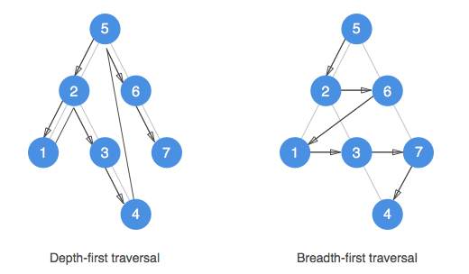 Depth First and Breadth First tree walking
 So, how do we do that iteratively ? Since we can only perform either left or right partition at a time, we need to store all the ranges that we need to perform next.
But, since we only need to know ranges that had not yet been partitioned, we can reuse indexes.
Here is what we will do while we loop through the tree :
- when a node is being partitioned, it will be removed from the array.
- after partitioning, the corresponding ranges for left and right children will be stored into the array.
Here is a demo :
// 1. initially, we will store the low and high values
// before partition
    [ 5, 9, 3, 1, 2, 8, 7, 6 ] // low = 0, high = 7
    [ 0, 7 ]                   // stack [ low, high ]
     └-┬--┘
       └--- low and high index that partition is acting on

// 2. First Partition
// when partition is performed, we need to erase
// the parent's data, and store the children's data.
    [ 5, 3, 1, 2, 6, 8, 7, 9 ] // p = 4
// remove node [ 0 , 7 ]
    [ 5, 7, 0, 3 ]
     └-----┬----┘
           └------- calculated low and high indexes of children

// 3. Second Partition on [ 0, 3 ]
// same will happen on the second partition
    [ 5, 3, 1, 2 ] -> [ 1, 2, 5, 3 ] // p = 1
    [ 5, 7, 0, 3 ]                   // stack
            └-┬-┘
              └--- low and high index that is acting on

// remove node [ 0 , 3 ]
    [ 5, 7, 2, 3, 0, 0 ]
            └----┬-----┘
                 └------- low and high indexes for children

... this will continue until all nodes have been visited
With these in mind, here’s how we write in code :
void quicksort (int arr[], int low, int high) {
    if (low >= high || low < 0) return;
    int ranges[high - low + 1];
    int currentIndex = -1;

    // initial partition
    ranges[++currentIndex] = low;
    ranges[++currentIndex] = high;

    while(top >= 0) {
        // fetch parent's node data
        high = ranges[currentIndex--];
        low = ranges[currentIndex--];

        if (low >= high || low < 0) continue;

        int p = partition(arr, low, high);

        // store children's data
        ranges[currentIndex++] = p + 1;
        ranges[currentIndex++] = high;

        ranges[currentIndex++] = low;
        ranges[currentIndex++] = p - 1;

    }
}
Time Complexity
From our experience in Heap Sort and Merge Sort, we would expect the time complexity to be $O(nlog(n))$. But that is not the case.
If we look at sorting process :
void recursiveSort(int arr[], int low, int high) {
    if (low < 0 || low >= high) return;

    int p = partition(arr, low, high);

    recursiveSort(arr, low, p - 1);
    recursiveSort(arr, p + 1, high);
}
we can see that it works the same as Heap Sort.
But that’s only if our pivots are all located at the center of the array.
Let’s take a look at what will happen when the input array is either inversed or reversed :
                             [1, 2, 3, 4, 5]    level 1
                           ┌--------┴-------┐
                     [1, 2, 3, 4]   5      [ ]  level 2
                  ┌--------┴-------┐
              [1, 2, 3]    4      [ ]           level 3
         ┌--------┴-------┐
      [1, 2]      3      [ ]                    level 4
  ┌-----┴------┐
 [1]    2     [ ]                               level 5
As you can see, the tree’s height is not $log(n)$, but $n$. Thus, the worst case time complexity is :
\[\text{worst case} = O(n^2)\]So how can we improve this ? To improve this, we need to choose pivots that can best divide the array in half in each level.
This can be done through randomly selecting values as pivot.
Space Complexity
Space complexity differs in both iteration and recursion implementations.
Iteration In iterative implementation, the only space we need is the stack that stores calculated low and high values.
If we look at the code in the while loop :
// fetch parent's node data
high = ranges[currentIndex--];
low = ranges[currentIndex--];

if (low >= high || low < 0) continue;

int p = partition(arr, low, high);

// store children's data
ranges[currentIndex++] = p + 1;
ranges[currentIndex++] = high;

ranges[currentIndex++] = low;
ranges[currentIndex++] = p - 1;
In every loop, the size of the stack will increase by :
\[\text{space increment} = -2 + 2 + 2 = 2\]And since the maximum height of the tree is $n$, the total space complexity in the worst case is :
\[\text{space complexity}_\text{worst case} = 2n = O(n)\]However, if the pivot were to be chosen randomly, then :
\[\text{space complexity}_\text{best case} = 2log(n) = O(log(n))\]Source Code
C++ Recursive
static void recursiveSort(vector<int>& nums, int low, int high) {

    if (low >= high || low < 0) return;

    int pivot = partition(nums, low, high);

    recursiveSort(nums, low, pivot - 1);
    recursiveSort(nums, pivot + 1, high);
}

static int partition(vector<int>& nums, int low, int high) {

    int pivot = nums[high];
    int i = low - 1;

    for (int j = low; j < high; j++) {
        if (nums[j] <= pivot) {
            i++;
            swap(nums, i, j);
        }
    }

    i++;
    swap(nums, i, high);
    return i;
}
C++ Iterative
static void iterativeSort(vector<int>& nums, int low, int high) {
    if (low >= high || low < 0) return;
    stack<int> ranges;

    ranges.push(low);
    ranges.push(high);

    while(ranges.size() > 0) {
        high = ranges.top();
        ranges.pop();
        low = ranges.top();
        ranges.pop();

        if (low >= high || low < 0) continue;

        int p = partition(nums, low, high);

        ranges.push(p + 1);
        ranges.push(high);

        ranges.push(low);
        ranges.push(p - 1);
    }
}

static int partition(vector<int>& nums, int low, int high) {

    int pivot = nums[high];
    int i = low - 1;

    for (int j = low; j < high; j++) {
        if (nums[j] <= pivot) {
            i++;
            swap(nums, i, j);
        }
    }

    i++;
    swap(nums, i, high);
    return i;
}
C++ Iterative (Optimized)
static void iterativeSort(vector<int>& nums, int low, int high) {
    if (low >= high || low < 0) return;
    stack<int> ranges;

    ranges.push(low);
    ranges.push(high);

    while(ranges.size() > 0) {
        high = ranges.top();
        ranges.pop();
        low = ranges.top();
        ranges.pop();

        int p = partition(nums, low, high);

        if (p + 1 < high) {
            ranges.push(p + 1);
            ranges.push(high);
        }

        if (p - 1 >= low) {
            ranges.push(low);
            ranges.push(p - 1);
        }
    }
}

static int partition(vector<int>& nums, int low, int high) {

    int pivot = nums[high];
    int i = low - 1;

    for (int j = low; j < high; j++) {
        if (nums[j] <= pivot) {
            i++;
            swap(nums, i, j);
        }
    }

    i++;
    swap(nums, i, high);
    return i;
}
Reference
Counting Sort
Counting Sort is the first non-comparison sort that we will learn.
It is a linear time sorting algorithm that uses key-value data structure to store the values from the array as key and the number of values that are smaller than or equal to a specific number as value.
Counting Sort can only be applied to positive integers, meaning :
- the input array $A[1:n]$ must contain values ranges from $0\text{ to }k$, where $k$ is a non-negative integer.
Now, to perform Counting Sort, we need to do the following steps :
- find the maximum value ( $k$ ) in the array
- create a new array, $C[0:k]$, that holds only zeros.
- loop through the input array $A[1:n]$ and increment the value of $C[A[i]]$ by 1
- by the end, $C[0:k]$ will store the number of times $A[i]$ occurs in $A[1:n]$
- loop through $C[0:k]$ and perform $C[i] = C[i] + C[i - 1]$
- $C[i]$ should now stores the number of values that are smaller than $i$, which is basically the sorted index for the value.
- create a new array, $B[1:n]$, to store the output by looping through $C[0:k]$.
These steps might be a bit unclear on how Counting Sort is performed, but the demo will clear things up for you.
Demo
Let’s perform Counting Sort on [ 5, 3, 1, 2, 9, 8, 7, 6, 1, 4, 7 ]
PS : the input array is seen as $A[1:n]$
| \(i\) | 1 | 2 | 3 | 4 | 5 | 6 | 7 | 8 | 9 | 10 | 11 |
|---|---|---|---|---|---|---|---|---|---|---|---|
| \(A[i]\) | 5 | 3 | 1 | 2 | 9 | 8 | 7 | 6 | 1 | 4 | 7 |
Following the steps, let’s create an array $C[0:k]$, where $k = 9$ :
| \(i\) | 0 | 1 | 2 | 3 | 4 | 5 | 6 | 7 | 8 | 9 |
|---|---|---|---|---|---|---|---|---|---|---|
| \(C[i]\) | 0 | 0 | 0 | 0 | 0 | 0 | 0 | 0 | 0 | 0 |
Next, we will loop through $A[1:n]$ and update values in $C[0:k]$
[ 5, 3, 1, 2, 9, 8, 7, 6, 1, 4, 7 ] → increment at index 5
\(i\) 0 1 2 3 4 5 6 7 8 9 \(C[i]\) 0 0 0 0 0 1 0 0 0 0 [ 5, 3, 1, 2, 9, 8, 7, 6, 1, 4, 7 ] → increment at index 3
\(i\) 0 1 2 3 4 5 6 7 8 9 \(C[i]\) 0 0 0 1 0 1 0 0 0 0 [ 5, 3, 1, 2, 9, 8, 7, 6, 1, 4, 7 ] → and so forth
\(i\) 0 1 2 3 4 5 6 7 8 9 \(C[i]\) 0 1 0 1 0 1 0 0 0 0 after looping through [ 5, 3, 1, 2, 9, 8, 7, 6, 1, 4, 7 ], we’ll get :
\(i\) 0 1 2 3 4 5 6 7 8 9 \(C[i]\) 0 2 1 1 1 1 1 2 1 1 loop through $C[0:k]$ to get the number of values smaller than or equal to $i$ :
\(i\) 0 1 2 3 4 5 6 7 8 9 \(C[i]\) 0 2 1 1 1 1 1 2 1 1 \(C[i]\) 0 2 3 1 1 1 1 2 1 1 \(C[i]\) 0 2 3 4 1 1 1 2 1 1 \(C[i]\) 0 2 3 4 5 6 7 9 10 11 create a new array $B[1:n]$ and loop through $C[0:k]$ using the values from $A[1:n]$ as the index :
\(i\) 1 2 3 4 5 6 7 8 9 10 11 \(A[i]\) 5 3 1 2 9 8 7 6 1 4 7 \(C[A[i]]\) 6 4 2 3 11 10 9 7 2 5 9
Here is what happen while loop through $n\text{ to }1$Step \(i\) \(A[i]\) \(C[A[i]]\) \(B[C[A[i]]] = A[i]\) \(C[A[i]] = C[A[i]] - 1\) 1 11 7 9 \(B[9] = 7\) \(C[7] = 8\) 2 10 4 5 \(B[5] = 4\) \(C[4] = 4\) 3 9 1 2 \(B[2] = 1\) \(C[1] = 1\) 4 8 6 7 \(B[7] = 6\) \(C[6] = 6\) 5 7 7 8 \(B[8] = 7\) \(C[7] = 7\) 6 6 8 10 \(B[10] = 8\) \(C[8] = 9\) 7 5 9 11 \(B[11] = 9\) \(C[9] = 10\) 8 4 2 3 \(B[3] = 2\) \(C[2] = 2\) 9 3 1 1 \(B[1] = 1\) \(C[1] = 0\) 10 2 3 4 \(B[4] = 3\) \(C[3] = 3\) 11 1 5 6 \(B[6] = 5\) \(C[5] = 5\) By the end, we will get $B[1:n]$ to be :
\[B[1:n] = \{ 1, 1, 2, 3, 4, 5, 6, 7, 7, 8, 9 \}\]And $C[0:k]$ changed from : \(\begin{aligned} C[0:k] &= \{ 0, 2, 3, 4, 5, 6, 7, 9, 10, 11 \} \end{aligned}\)
To :
\[\begin{aligned} C[0:k] &= \{ 0, 0, 2, 3, 4, 5, 6, 7, 9, 10 \} \end{aligned}\]
As you can see from the demo, $C[0:k]$ uses index to indicate the value, which acts as a key.
And the value stored in $C[0:k]$ is the corresponding index in $A[1:n]$.
PsudoCode
void countingSort(int arr[], int n, int k) {
    int b[n], c[k + 1];

    for i from 0 to k {
        c[i] = 0;
    }

    for i from 0 to n - 1 {
        c[arr[i]] = c[arr[i]] + 1;
    }

    for i from 1 to k {
        c[i] = c[i] + c[i - 1];
    }

    for i from 0 to n - 1 {
        b[c[arr[i]] - 1] = arr[i];
        c[arr[i]] = c[arr[i]] - 1;
    }

    for i from 0 to n - 1 {
        arr[i] = b[i];
    }
}
Time Complexity
The time complexity for Counting Sort is quite straight forward.
Since it consist of 4 or 5 loops that takes either $k$ or $n$ steps, the time complexity is $O(n + k)$.
Space Complexity
As you can see from the code, Counting Sort is not an in-place sorting algorithm, though it is a stable algorithm.
Instead of sorting the array in-place, Counting Sort uses $B[1:n]$ and $C[0:k]$ to store the sorted array and the key:values relationships, respectively.
Thus, the space complexity for Counting Sort is $O(n + k)$.
Source Code
C++
void iterationSort(vector<int>& arr, int n, int k) {
    int b[n]; int c[k + 1];

    for (int i = 0; i <= k; i++) {
        c[i] = 0;
    }

    for (int i = 0; i < n; i++) {
        c[arr[i]] = c[arr[i]] + 1;
    }

    for (int i = 1; i <= k; i++) {
        c[i] = c[i] + c[i - 1];
    }

    for (int i = 0; i < n; i++) {
        b[c[arr[i]] - 1] = arr[i];
        c[arr[i]] = c[arr[i]] - 1;
    }

    for (int i = 0; i < n; i++) {
        arr[i] = b[i];
    }
}
Characteristics
The characteristics of Counting Sort include :
- it is only suitable for arrays that only hold positive integers
- it does not rely on comparison to sort the array, instead, it uses key-value relationship to sort.
- it is not an in-place algorithm, it has a space complexity of $O(n + k)$
Bucket Sort
Bucket Sort aka Bin Sort is a non-comparison sorting algorithm that works by distributing the elements of an array into a number of buckets [wiki].A bucket is an array that contains values that are within certain range.
In order to perform Bucket Sort, we need to know the ranges the input array contains.
Bucket Sort works as follows :
- create an array of empty “bucket”
- Scatter : put values from the input array into their corresponding bucket
- Sort : sort all the non-empty buckets
- Gather : visit buckets in order and put all elements back into original array.
Demo
Let’s try to sort [ 19, 39, 3, 23, 20, 31, 17, 6 ] using Radix Sort.
create buckets :
range 0-9 10-19 20-29 30-39 [ ] [ ] [ ] [ ] Here we set the range for each bucket to be 10.
If you are not sure what value should be used, you can calculate it as follows :
\[range = \frac{(max - min)}{n}\]Since in the worst scenario, every bucket only contains a single value, thus the number of bucket can be set as the size of the input array.
\[range = \frac{(max - min)}{n} + 1\]
However, we need to add an extra 1 to take care of the last bucket.Scatter :
range 0-9 10-19 20-29 30-39 [ 3, 6 ] [ 19, 17 ] [ 23, 20 ] [ 39, 31 ] Sort :
range 0-9 10-19 20-29 30-39 [ 3, 6 ] [ 17, 19 ] [ 20, 23 ] [ 31, 39 ] Gether : [ 3, 6, 17, 19, 20, 23, 31, 39 ]
Now, you should be wondering, how do we sort each bucket ?
You can use any sorting algorithm that best suits your need.
PsudoCode
Here is what I think the sorting funtion should look like :
void sort(int arr[], int step, int min, int max)
However, that’s not correct, because in the worst scenario, there will be n buckets. So, we can assume there are n buckets to begin with.
In this psudocode we assume the input array only contains positive values.
void sort(int arr[], int min, int max) {
    int n = sizeof(arr)/sizeof(arr[0]);
    int range = (max - min)/n + 1;

    vector<int> buckets[n];

    for i from 1 to n {
        int v = arr[i];
        int index = ((v - min) / range);
        buckets[index].push_back(v);
    }

    for i from 1 to n {
        bucketSort(buckets[i]);
    }

    int curIndex = 0;
    for i from 1 to n {
        int bucketSize = buckets[i].size();
        for j from 1 to bucketSize {
            arr[curIndex] = buckets[i][j];
            currInd ++;
        }
    }
}
Time Complexity
As we can see, the code consist of 3 sections :
- Scatter
- Sorting
- Gather
Since scatter only need a single for-loop that runs n loops, therefore, it has a time complexity of $O(n)$.
As for gather, since it simply read all the values from buckets, it also has a time complexity of $O(n)$.
Finally, sorting depends on the time complexity of the selected sorting algorithm, therefore :
\[T(n) = O(n) + \sum_{i = 1}^{n-1}(\text{ sort big-O})\]In our case, since we used Insertion Sort, we get :
\[\begin{aligned} &T(n) = O(n) + \sum_{i = 1}^{n-1}O(n_i^2) \\&\text{where } n_i \text{ is the size in the } i^{th} \text{ bucket.} \end{aligned}\]And since in the worst case scenario, Bucket Sort is simply the time complexity of the selected sorting algorithm, therefore, in our case, it is $O(n^2)$.
In the best case scenario, the array should already be sorted, thus :
\[T(n) = \Omega(n)\]However, if Insertion Sort is not used, then the time complexity will be linear : $\Omega(n + k)$
Finally, in the average case, values within the input array will be distributed evenly :
\[\text{elements per bucket} = \frac{n}{k}\]making the average time complexity :
\[\begin{aligned} T(n) &= \Omega(n + k) + k * \Omega(\frac{n^2}{k^2}) \\&= \Omega(n + k) + \Omega(\frac{n^2}{k}) \\&= \Omega(n + k + \frac{n^2}{k}) \end{aligned}\]Space Complexity
From the code, we know that we need $k$ number of buckets that holds all n number of values. Thus, the space complexity is $O(n + k)$.
Source Code
C++
void sort(vector<int>& nums, int min, int max) {
    int n = nums.size();
    int range = (max - min)/n + 1;

    vector<int> buckets[n];

    for (int i = 0; i < n; i++) {
        int v = nums[i];
        int index = ((v - min) / range);
        buckets[index].push_back(v);
    }

    for (int i = 0; i < n; i++) {
        bucketSort(buckets[i]);
    }

    int curIndex = 0;
    for (int i = 0; i < n; i++) {
        int bucketSize = buckets[i].size();
        for (int j = 0; j < bucketSize; j++) {
            nums[curIndex] = buckets[i][j];
            // cout << "[i][j] = " << i << ", " << j << " value " << nums[curIndex] << "\n";
            curIndex ++;
        }
    }
}
Bucket vs Counting Sort
Similarities :
- Both are not in-place algorithm
- Both are only suitable for positve values
Differences :
- Counting Sort is stable sorting algorithm, but Bucket Sort is only stable if the selected sorting algorithm is stable.
- Bucket Sort requires other sorting algorithm to sort the buckets, while Counting Sort does not need.
- Counting Sort has a linear time complexity while Bucket Sort does not.
Here are other additional infos :
- Bucket Sort is useful when input is *uniformly distributed and is most often used to sort uniformly distributed floating point values [3].
- If the values are not as uniformly distributed, then simply use comparison sorting algorithm that best suit the condition.
- Also, the range of buckets can actually have different intervels.
Reference
Radix Sort
Radix Sort is a sorting algorithm that is based on Bucket Sort. Instead of distributing values based on ranges, it distribute values based on radix.
Since it uses buckets, sometimes it can also be called Bucket Sort and Digit Sort.
Radix Sort sorts the elements by
- first grouping the individual digits of the same place value.
- Then, sort the elements according to their increasing/decreasing order.
Demo LSD
Let’s try to sort [ 195, 29, 3, 193, 20, 81, 17, 6 ] using Radix Sort.
There are two ways to sort the array, we can start by the Least Significant Digit (LSD) or the Most Significant Digit (MSD).
Here is how the array is sorted starting from LSD
| buckets | 0 | 1 | 3 | 5 | 6 | 7 | 9 |
|---|---|---|---|---|---|---|---|
| values | 20 | 81 | 3 193 | 195 | 6 | 17 | 29 |
After gathering, we will get :
\[[20, 81, 3, 193, 195, 6, 17, 29]\]Then we will move to the second LSD :
| buckets | 0 | 1 | 2 | 8 | 9 |
|---|---|---|---|---|---|
| values | 03 06 | 17 | 20 29 | 81 | 193 195 |
Again, after gathering, we will get :
\[[3, 6, 17, 20, 29, 81, 193, 195]\]Though the array is sorted, but we will still go through the last radix :
| buckets | 0 | 1 |
|---|---|---|
| values | 003 006 017 020 029 081 | 193 195 |
Finally, we will get :
\[[3, 6, 17, 20, 29, 81, 193, 195]\]PsudoCode for LSD
void sort(int arr[], int max) {
    // 0 to 9
    node** buckets = new node*[10];
    int radix = 1;

    while(radix < max) {
        // scatter
        for i from 1 to n {
            int remainder = (arr[i] / radix) % 10;
            append(buckets[remainder], arr[i]);
        }

        // gather
        int index = 1;
        for i from 1 to 10 {
            while(!buckets[i] == NULL) {
                arr[index++] = pop(buckets[i]);
            }
        }
    }
}
Demo MSD
Now that we’ve seen how values are sorted using LSD, let’s take a look at how it works using MSD.
\[\text{input : }[ 195, 29, 3, 193, 20, 81, 17, 6 ]\]
Note : MSD does not go through the same process as LSD, as demostrates below.
Incorrect way to perform **Radix Sort** for MSD :
| buckets | 0 | 1 |
|---|---|---|
| values | 029 003 020 081 017 006 | 195 193 |
After we gather :
\[[29,3,20,81,17,6,195,193]\]| buckets | 0 | 1 | 2 | 8 | 9 |
|---|---|---|---|---|---|
| values | 03 06 | 17 | 29 20 | 81 | 195 193 |
Then we will get :
\[[3, 6, 17, 29, 20, 81, 195, 193]\]Finally :
| buckets | 0 | 1 | 3 | 5 | 6 | 7 | 9 |
|---|---|---|---|---|---|---|---|
| values | 20 | 81 | 3 193 | 195 | 6 | 17 | 29 |
We will get :
\[[20, 81, 3, 193, 195, 6, 17, 29]\]Hm, that’s not what we expected. So what’s going on ?
At the first step when we are sorting with MSD, all values are already placed at their final location, or at least the final bucket.
Therefore, instead of rearranging all values again in buckets, we simply need to sort values within the same bucket with a new set of buckets :
Here is how Sorting is done using MSD
          [ 195, 29, 3, 193, 20, 81, 17, 6 ]
                   0       |       1
                   ┌-------┴-------┐
                  029             195
                  003             193
                  020              |
                  081              |
                  017              |
                  006              |
          0    1   |   2   8       |
          ┌----┬---┴---┬---┐       | 9
         03   17      29   81     195
         06    |      20   |      193
        3 | 6  |     0 | 9 |     3 | 5
        ┌-┴-┐  |7    ┌-┴-┐ |1    ┌-┴-┐
        3   6  17   20  29 81   193 195
        |   |  |    |   |  |    |   |

       [ 3, 6, 17, 20, 29, 81, 193, 195 ]
PsudoCode for MSD
The easiest way to implement MSD Radix Sort is to use recursion.
void msdSort(int targetArr[], int finalArr[], int radix, int index) {
    node** buckets = new node*[10];

    for i from 1 to 10 {
        INITIALIZE node*
    }

    for i from 1 to targetN {
        append(buckets[targetArr[i] / radix % 10], targetArr[i]);
    }

    if (radix == 1) {
        int currentIndex = index;
        for i from 1 to 10 {
            while(buckets[i] != NULL) {
                finalArr[currentIndex++] = popFirst(buckets[i]);
            }
        }
    } else {
        for 1 from 1 to 10 {
            vector<int> nextArr;
            while(buckets[i] != NULL) {
                nextArr.push_back(popFirst(buckets[i]));
            }

            if (nextArr.size() > 0) {
                int arr[nextArr.size()];
                copy(nextArr.begin(), nextArr.end(), arr);
                msdSort(arr, finalArr, radix / 10, index);
                index += nextArr.size();
                nextArr.clear();
            }
        }
    }
}
Time Complexity
The time complexity for LSD approach is quite straight forward.
The LSD approach consist of 3 loops :
- a while-loop that changes the radix ($10^0, 10^1, 10^2 … 10^r$)
- a for-loop that goes from 1 to n
- a for-loop that goes through all buckets ($b$)
If we know the maximum value in the input array to be $k$, then we can be calculate $r$ as follows :
\[r = log_{10}k\]Thus, LSD approach has a time complexity of $O(r(n + b))$ for all cases.
If $r$ is a constant and $b = O(n)$, then this will make LSD approach a linear time run.
As for the time complexity for MSD approach, though it is quite different from LSD approach, it also has time complexity of $O(r(n+b))$.
Space Complexity
Since in our case, Radix Sort is not an in-place sorting algorithm, it will need $O(n+k)$ space complexity.
Source Code
C++ LSD with Vector
void lsdSortVector(vector<int>& nums, int max) {
    // 0 to 9
    vector<int> buckets[10];
    int counters[10] = { 0 };
    int radix = 1;

    while(radix < max) {

        for (int i = 0; i < nums.size(); i++) {
            int v = nums[i];
            int di = nums[i] / radix;
            int bucket = di % 10;
            buckets[bucket].push_back(v);
            counters[bucket] += 1;
        }

        // gather
        int index = 0;
        for (int i = 0; i < 10; i++) {
            for (int j = 0; j < counters[i]; j++) {
                nums[index] = buckets[i][j];
                index ++;
            }
        }

        for (int i = 0; i < 10; i++) {
            while(!buckets[i].empty()) {
                buckets[i].pop_back();
            }
        }

        fill(begin(counters), end(counters), 0);

        radix *= 10;
    }
}
C++ LSD with LinkedList
void lsdSortLinkList(vector<int>& nums, int max) {
    // create buckets
    node** buckets = new node*[10];
    int radix = 1;

    // init
    for (int i = 0; i < 10; i++) {
        buckets[i] = nullptr;
    }

    while(radix < max) {
        for (int i = 0; i < nums.size(); i++) {
            int bucket = (nums[i] / radix) % 10;
            append(buckets[bucket], nums[i]);
        }

        int bucket = 0;
        int index = 0;
        while(bucket < 10) {
            while(buckets[bucket] != nullptr) {
                nums[index++] = popFirst(buckets[bucket]);
            }
            bucket++;
        }

        radix *= 10;
    }
}

/**
 * @brief Below contains all class and fucntions for link list
 *
 */
// Node : https://www.geeksforgeeks.org/radix-sort/
struct node {
    int data;
    node* next;
};

struct node* create(int data) {
    node* temp = new node();
    temp->data = data;
    temp->next = nullptr;
    return temp;
}

void append(node*& header, int data) {
    if(header == nullptr) {
        header = create(data);
        return;
    }

    node* t = header;

    while(t->next != nullptr) {
        t = t->next;
    }
    t->next = create(data);
}

int popFirst(node*& header) {

    if (header == nullptr) {
        return 0;
    }

    node* t = header;
    int data = t->data;

    header = header->next;

    delete t;
    return data;
}
C++ MSD with LinkedList
void msdSort(vector<int>& nums, vector<int>& original, int radix, int index) {

    if (radix == 0) return;

    node**buckets = new node*[10];

    for (int i = 0; i < 10; i++) {
        buckets[i] = nullptr;
    }

    // scatter
    for (int i = 0; i < nums.size(); i++) {
        append(buckets[(nums[i] / radix) % 10], nums[i]);
    }

    if (radix == 1) {
        int currentIndex = index;
        for (int i = 0; i < 10; i++) {
            while(buckets[i] != nullptr) {
                original[currentIndex++] = popFirst(buckets[i]);
            }
        }

        cout << '{';
        for (auto i : original) {
            cout << i << ", ";
        }
        cout << "}\n";
    } else {
        int nextIndex = index;
        for(int i = 0; i < 10; i++) {
            vector<int> nextNum;

            while(buckets[i] != nullptr) {
                nextNum.push_back(popFirst(buckets[i]));
            }

            if (!nextNum.empty()) {
                msdSort(nextNum, original, radix / 10, nextIndex);
                nextIndex += nextNum.size();
                nextNum.clear();
            }
        }
    }

}
Other implementations
In our current sample code, we uses Bucket Sort as subroutine in Radix Sort. However, we can also use Counting Sort approach to implement it.
Radix Sort vs Counting Sort vs Bucket Sort
From what we’ve seen so far, Radix Sort is just like Bucket Sort. Not only is Radix sorting data with buckets, but we can also use other sorting algorithms to sort items within a bucket.
Another thing, comparison based sorting algorithms have a lower bound of $O(nlog(n))$, while Counting Sort, a linear time sorting algorithm, has a time complexity of $O(n + k)$ when elements are in the range of $[1:k]$.
But, what if elements are in the range of $[1:n^2]$ ?
But when the range is greater than linear, such as $[1:n^2]$, Counting Sort would take $O(n^2)$ which is much slower than comparison sorting algorithms ( $O(nlog(n))$ ) but Radix Sort can solve it as linear complexity.
So Radix Sort is better than Counting Sort when the range is greater than linear.
Applications
Radix Sort dates back to 1890s when Herman Hollerith implements it on tabulating machines. It came into common use in 1923 as a way to sort punched cards.
Since Radix Sort is designed to sort data that can be sorted lexicographically, it can be used to sort :
- integers
- words
- punched cards
- playing cards
- mails
Reference
- Bucket-Sort and Radix-Sort pdf
- geek for geek
- programiz
- Counting Sort vs Radix Sort vs Bucket Sort
- Tabulating machine
Conclusion
In this post, we’ve covered 10 sorting algorithms.
Though there are many details that weren’t discussed, namely average time complexity and applications, but I hope this post gives you a basic insight on how different sorting algorithms different from one another.
Also, keep in mind that do not judge an algorithm just by time or space complexity, you need to find the one that best suit your needs.
If you have any suggestions or questions, please leave a message and I hope all of you find this post useful.
About Post
- Author:Jimmy Liu
- Link:https://kuopingl.github.io//2022/11/14/algo-sorting/
- Copyright:Free to share and adapt, but remember to give proper credit(CC BY-SA 3.0)